Laplace Equation
Posted on May 18, 2019 in Physics
The Laplace equation is:
Some physical applications where laplace equation arises naturally are:
- Steady state temperature distribution in the region with no source or sink
- Electrostatic potential in a region with no charge density
- Gravitational potential in a region with no mass
- Velocity potential in a region of fluid with no source or sink
Do you see some pattern here ? Of course you do!
But, before talking about any specific cases of these applications, let's talk about the equation itself. Let's see what kind of functions satisfy the Laplace equation.
Let's first look at one dimensional example. Laplace equation in one dimension is:
We can solve the equation:
Integrate twice to get:
which is an equation of a straight line, a and b being constants.
Before we look at higher dimension, let me assert some properties of this soultion:
-
the value of the function at a point is the average of the value at points around it.
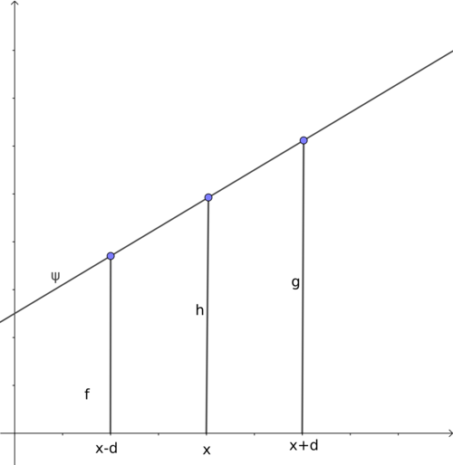
Take two points at equal distance on either side of any point x, the following relation holds:ψ(x)=12[ψ(x+d)+ψ(x−d)]
where, d is any distance. -
The solution has no local maxima or minima and the global minima and maxima always lie on the end points i.e. on the boundary.
These properties are easy to verify on a straight line. But they also apply to higher dimensions.
Now let's look at 2D case. Laplace equation in two dimension is:
This is no longer an ordinary differential equation. It is impossible to write a complete general solution (in closed form) to this second order partial differential equation.
But we can get some idea about the nature of the solution.
Again, the value at any point should be the average of the value of the function at neighboring points i.e. in case of 2D, points at a circle of radius R around the point. And therefore,
And the function which is a 2 dimensional surface on a 3D space (x and y as input space and z as the output) would have no local minima or local maxima.
Why? Well, you can see from the equation itself that second derivative with respect to x and y should have opposite signs. That means if the surface is concave downward in x direction at some point, it has to be concave upward along y direction at that point. That implies the point can't be a local minima or a local maxima.
To solidify this understanding, imagine a hollow pipe like this:

Now, chip away at the upper end of the cylinder creating a topography however you like. You're deciding on the boundary conditions. Now imagine covering this undulating end of the pipe with stretchable rubber sheet tightly such that the sheet touches the cylinder at every point on the boundary.
The surface of the rubber gives you a solution of the Laplace equation with the boundary condition you specified. Realize that such rubber surface would have no peaks or valley inside the boundary.
Does this make sense ?
As physicist, our job is to ask ourselves if this property we highlighted makes sense for all the physical application where Laplace equation comes about.
We can be sure that it does by using symmetry argument.
Consider a metal rod of finite length l with ends kept at 0 °C and 100 °C as in figure below. We are interested in the steady state temperature i.e. the temperature distribution in the rod after a long time such that it doesn't change further as time evolves.
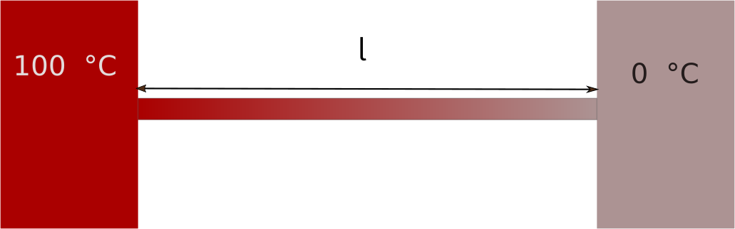
Take any point along the rod, what the property #1 tells us is that the temperature at this point is the average of the temperature immediately next to it. Which is reasonable, right ?
Because, part of the rod on one side is trying to cool the point and part of the rod on other side is trying to heat it up and the point eventually has to "make peace" with the both sides, and settle on the average temperature which doesn't change further.
This is true for every point in the rod except, of course, the end points.
The second point was that there are no local minima/maxima on the inside of the rod.
Suppose there is a local minima at a point within the rod somewhere. That implies the temperature of the rod on both sides is higher that the temperature at this point. We know for sure this can't happen. Why? Because If this were the case, the point would start to be heated from both sides and the temperature would start to change. But this can't happen since we're already talking about steady state temperature. All the temperature needs to happen, has already happened before arriving at the steady state.
You can argue similarly for local maxima.
Velocity potential, electrostatic and gravitational potential can be understood similarly.
If the fluid velocity potential distribution in the region wasn't like we characterized above, then there would be net force across the region to cancel out these irregularities and the system would reach this 'smoothness' asymptotically.
Note that the condition would be entirely different, if there were sources or sinks within the rod. Sources would heat up the rod on both sides and thus create maxima and sinks would create minima. In fact, Laplace equation doesn't hold such cases. There would be non zero source/sink term on the RHS to account for these sources/sinks. This equation is called Poission's equation.
where f(x,y,z) characterizes the sources/sinks in the space. This could be charge density in electrostatics, mass density in gravitation.
The End.